Kalman Filter

A comprehensive 2D Kalman filter tutorial for self_t+dt and any explorer from space time.

A beautiful picture of a lion laughing (maybe) which makes absolutely no sense at all here, just as much sense kalman filter did to me before I decided to write this guide

Introduction

From car navigation systems, autopilots to brain-computer interfaces or even landing humans on the moon (Apollo 11 lunar module) the kalman filter is a ingenious tool that combines uncertain information about systems to produce an accurate guess of the system's state. Kalman filter finds its use in dynamic systems that have some uncertain information about their state and helps in making an educated guess about its current state using measurements which are usually obtained from noisy sensors. Why noisy sensors you ask? because reality my friend!

Objectives

To understand the intuition behind kalman filters.
To design a kalman filter to track the position and orientation of a robot moving on a 2D plane with 3 degrees of freedom (translation in x, translation in y and angular rotation along z or yaw).
To understand sensor fusion using kalman filters.
To be able to design application specific kalman filters.

Gaussian distribution and product of 2 gaussian PDFs

Before we dive in, lets understand how probability distribution functions (PDFs) work, which form the basis of the mathematics we will be looking later in this article

For 2 normally (Gaussian) distributed functions we define the probability density functions with means $\mu_1, \mu_2$ and variances $\sigma_1^2, \sigma_2^2$

the mean ( $\mu$ ) in our case is the position where we expect the robot to be, while the variance ( $\sigma^2$ ) signifies how far the spread of this value is.

$\newline x_1(t) = \frac{1}{\sqrt{2\pi\sigma_1^2}}e^{-\frac{(t-\mu_1)^2}{2\sigma_1^2}} \\ \newline x_2(t) = \frac{1}{\sqrt{2\pi\sigma_2^2}}e^{-\frac{(t-\mu_2)^2}{2\sigma_2^2}}$

The product of the gaussian function above will have mean and variance given as

$\newline \mu = \frac{\frac{\mu_1}{2\sigma_1^2} + \frac{\mu_2}{2\sigma_2^2}}{\frac{1}{2\sigma_1^2} + \frac{1}{2\sigma_2^2}} = \frac{\mu_1\sigma_2^2 + \mu_2\sigma_1^2}{\sigma_2^2 + \sigma_1^2} \\ \newline \newline \sigma^2 = \sigma_1^2 \sigma_2^2 = \frac{1}{\frac{1}{\sigma_1^2} + \frac{1}{\sigma_2^2}} = \frac{\sigma_1^2\sigma_2^2}{\sigma_1^2 + \sigma_2^2}$

we use these equations to correct the predicted value by the system dynamic model using the measurement as depicted in the graph below

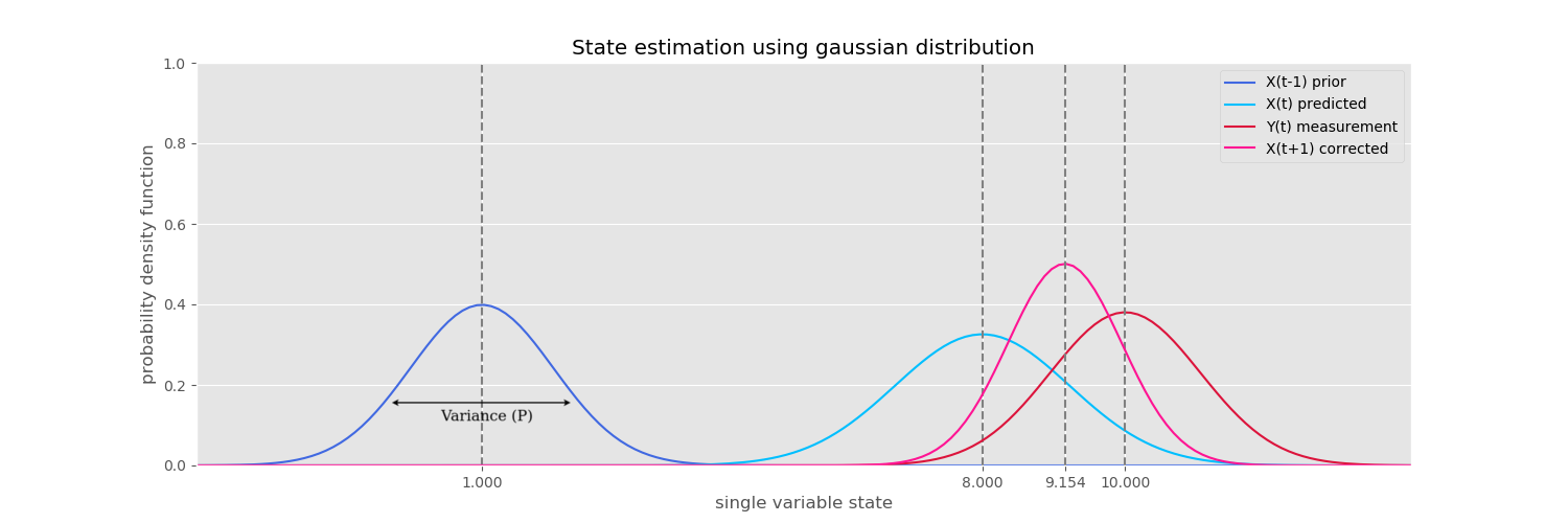
State estimation using gaussian distribution

As a thought experiment imagine a robot that moves in 1 dimension only (x). which has a 1D position sensor. The prior is where we assume our robot started at and has a high variance value (P). The mean/position is 1.0 units but the high variance implies our value could be somewhere around 1.0 with a high chance of being 1.0. We predict the robot position in time given the velocity at 1.0 to be at at 8.0 but as can be seen has a bigger spread than the prior value as the predictions will be noisy based on the chosen system model (we 'guess' the position hence we add more noise). A position sensor measurement is found to be 10.0 and has a slightly lower spread. The resultant product of the measured and predicted values is a gaussian which is the corrected value, the location of which can be found using the mean formula above (9.154) and the spread using the variance formula. From the plots we see that the resultant has a lower spread than both the predicted and measured value which essentially means we are now more certain about the position of the robot than what we started with (prior). This corrected value becomes the prior for the next prediction and the cycle continues till sensor measurements are coming in and we get an accurate location of the robot. This is the basic principle behind kalman filter.

Algorithm

In this section we will look at the functional block diagram of kalman filters.

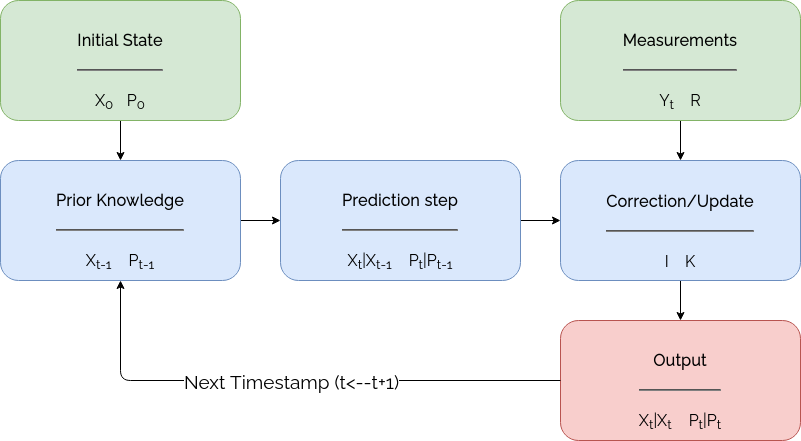
Block diagram of kalman filter

The initial state of the system is given as the first input to the kalman filter. $X_0$ is the state with position, velocity and/or acceleration values. Which can be set to all 0 if not known. $P_0$ is the initial system noise and the diagonals are set to very high values if the state is not known accurately. The intuition is that we declare the system state (position and velocity) is zero but we are highly uncertain about our estimate and hence the high covariance values in the $P$ matrix.
The first input then becomes the prior knowledge of state in the kalman filter and will be updated continuously as new measurements come into the system.
The prediction step predicts the next state of the system given the current state. The system noise is added to the $P$ matrix at this stage.
Measurements are then used to correct the system state using the kalman gain computed using the system and sensor noise matrices. The noise estimate now is also updated and will reduce if a high kalman gain was obtained.
The newly corrected state and noise estimate now can be observed as the new position of the system (robot) and in unit time will become the prior for predicting the next state of the system. This process continues till the system runs and new measurements are taken in from the sensors.

Now that we have a roadmap to what we want to achieve lets get deeper into the math. The following sections will explain how the system and sensors are modelled before we apply the kalman filter equations.

Dynamic model

The next set of equations of motion describe the motion of the robot with acceptable accuracy (neglecting the higher order differentials of the Taylor series approximation like jerk (literally!)).

the position of the object in unit time (t+1) given the velocity and acceleration can be predicted as...

$\begin{align*} \newline x_{t+1} &= x_t + t\dot{x}_t + \frac{t^2}{2}\ddot{x}_t \\ \newline y_{t+1} &= y_t + t\dot{y}_t + \frac{t^2}{2}\ddot{y}_t \\ \newline \theta_{t+1} &= \theta_t + t\dot{\theta}_t + \frac{t^2}{2}\ddot{\theta}_t \\ \newline \dot{x}_t = \frac{dx_t}{dt} &= \text{Object velocity along x at time t} \\ \newline \ddot{x}_t = \frac{d^2x_t}{dt^2} &= \text{Object acceleration along x at time t} \\ \end{align*}$

the velocity can be estimated as...

$\large \newline \dot{x}_{t+1} = \dot{x}_t + t\ddot{x}_{t} \\ \newline \dot{y}_{t+1} = \dot{y}_t + t\ddot{y}_{t} \\ \newline \dot{\theta}_{t+1} = \dot{\theta}_t + t\ddot{\theta}_{t} \\$

The above motion equations can be represented as a system dynamics matrix. The system state in this case is the position (x, y, orientation or heading angle which is 0 if heading parallel to x axis) and velocity (linear along x and y, angular along z)

$\large X_{n+1} = \begin{bmatrix} x_{n+1} \\ y_{n+1} \\ \theta_{n+1} \\ \dot{x}_{n+1} \\ \dot{y}_{n+1} \\ \dot{\theta}_{n+1} \end{bmatrix} = \begin{bmatrix} 1 & 0 & 0 & t & 0 & 0 \\ 0 & 1 & 0 & 0 & t & 0 \\ 0 & 0 & 1 & 0 & 0 & t \\ 0 & 0 & 0 & 1 & 0 & 0 \\ 0 & 0 & 0 & 0 & 1 & 0 \\ 0 & 0 & 0 & 0 & 0 & 1 \end{bmatrix} \begin{bmatrix} x_{n} \\ y_{n} \\ \theta_{n} \\ \dot{x}_{n} \\ \dot{y}_{n} \\ \dot{\theta}_{n} \end{bmatrix} + \begin{bmatrix} \frac{t^2}{2} & 0 & 0 \\ 0 & \frac{t^2}{2} & 0 \\ 0 & 0 & \frac{t^2}{2} \\ t & 0 & 0 \\ 0 & t & 0 \\ 0 & 0 & t \end{bmatrix} \begin{bmatrix} \ddot{x}_n \\ \ddot{y}_n \\ \ddot{\theta}_n \end{bmatrix}$

This state space representation can be equated as...

$\large X_{n+1} = AX_n + BU_n + w$

where

$\large A = \begin{bmatrix} 1 & 0 & 0 & t & 0 & 0 \\ 0 & 1 & 0 & 0 & t & 0 \\ 0 & 0 & 1 & 0 & 0 & t \\ 0 & 0 & 0 & 1 & 0 & 0 \\ 0 & 0 & 0 & 0 & 1 & 0 \\ 0 & 0 & 0 & 0 & 0 & 1 \end{bmatrix} \text{ } B = \begin{bmatrix} \frac{t^2}{2} & 0 & 0 \\ 0 & \frac{t^2}{2} & 0 \\ 0 & 0 & \frac{t^2}{2} \\ t & 0 & 0 \\ 0 & t & 0 \\ 0 & 0 & t \end{bmatrix}$

Matrix $A$ is the system dynamics matrix that aids in predicting the next state of the kalman filter given the current state. Matrix $B$ is the control input model and matrix $U$ is the control vector. If the system has any control inputs they can be modelled in these matrices to predict the next state and accordingly Q (described below) should be updated to account for the noise input (eg: A gas pedal could be given as a control input to estimate the acceleration in which case the B matrix remains as is, since acceleration is given as input).

$w$ represents the uncertainty or noise in the estimate of the system state as we exclude the higher order differentials in the system.

Process noise

The process noise $w$ is the noise which arises due to linearisation of the system model using the Taylor series expansion and causes error in prediction of system state given the current state. If accounting for a control input this noise will also represent the noise due to external factors on the system (eg: road friction and air drag on a car). Process noise can be modelled as an equation.

$\large Q = BQ_aB^T$

where $Q_a$ is the uncertainty or noise in the acceleration given as variance (square of standard deviation) of acceleration.

$\large Q_a = \begin{bmatrix} \sigma_{\ddot{x}}^2 & \sigma_{\ddot{y}}.\sigma_{\ddot{x}} & \sigma_{\ddot{\theta}}.\sigma_{\ddot{y}} \\ \sigma_{\ddot{x}}.\sigma_{\ddot{y}} & \sigma_{\ddot{y}}^2 & \sigma_{\ddot{\theta}}.\sigma_{\ddot{y}} \\ \sigma_{\ddot{x}}.\sigma_{\ddot{\theta}} & \sigma_{\ddot{y}}.\sigma_{\ddot{\theta}} & \sigma_{\ddot{\theta}}^2 \end{bmatrix}$

The matrix diagonals represent the variance (noise) in each predicted variable. The non diagonal values in the matrix represent the covariance between variables (eg: how noise in x is correlated to y is given in row 2 column 1 which is the same as row 1 and column 2). Assuming there is no correlation between the noise in acceleration of x to the noise in acceleration of y or $\theta$ we can write $Q_a$ by equating the non diagonal elements to 0.

$\large Q_a = \begin{bmatrix} \sigma_{\ddot{x}}^2 & 0 & 0 \\ 0 & \sigma_{\ddot{y}}^2 & 0 \\ 0 & 0 & \sigma_{\ddot{\theta}}^2 \end{bmatrix}$

Measurement model

Sensors (eg: GPS, imu) are modelled in this section which involves conversion of units or representation (polar to cartesian or cartesian to polar). The measurement equation can be written as.

$\large Y_{t+1} = H X_{t+1} + V$

The translation matrix $H$ allows the conversion of measurements (eg: units, polar or cartesian form) coming in from sensors to the form represented by the state space model.

in our case say we have a local gps system that sends us position updates in same units hence the value 1, this value will change if we use different units for measurement or if we have another representation of position like polar instead of cartesian coordinates.

the 3 rows indicate that we have 3 measurements x,y, $\theta$ coming from our local GPS while the 6 columns represent the states in our system. Since we don't measure velocity, these columns have value 0.

$\large H = \begin{bmatrix} 1 & 0 & 0 & 0 & 0 & 0\\ 0 & 1 & 0 & 0 & 0 & 0\\ 0 & 0 & 1 & 0 & 0 & 0 \end{bmatrix}$

Measurement noise

Thank Carl Friedrich Gauss for the normal distribution

As there are no perfect sensors we have to model the noise in the sensors. Sensor noise in kalman filters is assumed to be normally distributed hence is represented by the variance or the spread of the value measured by the sensors. Assuming that the measurement noise of the sensors in different dimensions is uncorrelated, we set our non diagonal values in the measurement noise matrix to zero.

$R = HH^TV \newline \newline V = \begin{bmatrix} \sigma_{x}^2 & 0 & 0 \\ 0 & \sigma_{y}^2 & 0 \\ 0 & 0 & \sigma_{{\theta}}^2 \end{bmatrix}$

hence in our case

$R = \begin{bmatrix} \sigma_{x}^2 & 0 & 0 \\ 0 & \sigma_{y}^2 & 0 \\ 0 & 0 & \sigma_{{\theta}}^2 \end{bmatrix}$

Now that we have modelled our system as well as the measurements coming into it we are ready to plug in our values into the kalman filter.

The algorithm consists of 3 crucial steps: Prediction, gain calculation and update

Prediction step

The next system state and noise in unit time can be predicted given the current state and system noise as below.

$\large \newline X_{t+1} = AX_t + BU \\ \newline P_{t+1} = AP_tA^{-1} + Q \\$

Kalman Gain (K)

Now we calculate the kalman gain $K$ . This value simply represents the proportion in which we should use our measurements versus our prediction to estimate our next state.

$K = \frac{P_tH^T}{HP_tH^T+R}$

The denominator for this equation $HP_tH^T+R$ is also known as the innovation and is denoted as $I$ hence the equation can be written as.

$\large \newline K = P_tH^TI^{-1} \\ \newline I = HP_tH^T+R \\$

The general intuition for kalman gain is as the equation below. Higher the noise in measurements the less we trust the external measurements w.r.t our predicted state hence lower the gain.

$\large $K = \frac{\text{System Noise (P)}}{\text{System Noise (P)} + \text{Measurement Noise (R)} }$$

Correction step

Here we update our system state using our predictions and measurements.

$\large $X_{t+1} = X_{t+1} + K[Y_{t+1} - HX_{t+1}]$$

All the step above does is to correct the value we had at prediction state using the kalman gain value we calculated

Put simply as the weighted average of measurement and prediction. Recall product of 2 PDFs

$\large $X_{corrected} = X_{predicted} + K(X_{measured} - X_{predicted})$$

$\large $X_{corrected} = K.X_{measured} + (1-K) X_{predicted}$$

The system noise is now corrected as.

$P_{t+1} = (I_6 - KH)P_{t+1}$

where

$I_6 = \text{Identity matrix of dimensions 6X6}$

Designing Kalman Filters

Designing an application specific kalman filter involves defining the correct matrices based on the chosen state space model and measurement model (sensors).

Kalman Filter (Constant velocity model)

The equations for kalman filter above will be used in this section to model a simple constant velocity model of kalman filter where we neglect acceleration and higher order terms for linearising the system. The only measurement given here will be from a position sensor (like GPS that monitors the robots position in x, y and yaw) that has some degree of inaccuracy.

The design method flows as follows

The state space model remains the same as we stated above

$X_{n} = \begin{bmatrix} x_{n} \\ y_{n} \\ \theta_{n} \\ \dot{x}_{n} \\ \dot{y}_{n} \\ \dot{\theta}_{n} \end{bmatrix}$

Dynamics matrix $A$ remains the same, matrix $B$ is not used for prediction since we provide no control input matrix $U$

Process noise matrix $Q$ will account for the noise due to neglecting acceleration and higher order differentials. It remains the same.

$\large Q_a = \begin{bmatrix} \sigma_{\ddot{x}}^2 & 0 & 0 \\ 0 & \sigma_{\ddot{y}}^2 & 0 \\ 0 & 0 & \sigma_{\ddot{\theta}}^2 \end{bmatrix}$

Measurement model needs matrix $H$ which remains the same as above since we have 6 state variables but we measure only 3 variables (x, y and theta) hence the shape 3x6

$\large H = \begin{bmatrix} 1 & 0 & 0 & 0 & 0 & 0\\ 0 & 1 & 0 & 0 & 0 & 0\\ 0 & 0 & 1 & 0 & 0 & 0 \end{bmatrix}$

The measurement noise input to the system will be from the position sensor and is modelled as.

$R = \begin{bmatrix} \sigma_{x}^2 & 0 & 0 \\ 0 & \sigma_{y}^2 & 0 \\ 0 & 0 & \sigma_{{\theta}}^2 \end{bmatrix}$

Once the above matrices have been defined the only work that is left is to plug in the values to the kalman filter algorithm. The prediction step is run and correction is performed when a measurement is available.

Legend for animations

The animations that follow show the kalman filters tracking a robot. The points below explain the color schemes and markers used in the plots.

The green line shows the real path the robot followed in the simulation which is a sine curve.
The corners on purple lines indicate the measurements from the position sensor, the discontinuities in this purple line indicate missing data from the position sensor (for mimicking loss of signal in GPS or asynchronous data).
The red dots indicate the position of robot as predicted by the kalman filter.
The arrows for respective plots indicate the orientation of the robot (yaw angle which is zero if the robot is parallel to the x axis).
Be advised that x coordinate in this animation has a linear relationship with time but has noise added hence will jump back and forth depending on the value. The y coordinate has a non linear relationship with time and hence the sine curve. Refer the modules/datagen.py section on the github repo for the motion model.
Plots later in this guide will have acceleration in x, y and theta and indicate the acceleration estimate of each variable at some timestamp. This plots are not given for the constant velocity model as they are not part of the state variable and hence cannot be observed.

kalman filter (constant velocity model) tracking robot position

The animation above was run on 100 timestamps with data missing at timestamps 10, 11, 12, 30, 31, 32, 33, 34, 50, 51 and 52. The initial state was set to x=0, y=0 and theta=0, also the velocities of respective variables were set to 0 as seen in the plot.
The predictions can be seen to overshoot at corners as we modelled our system as having constant velocity. At the corners the system cannot estimate that it is decelerating but just updates it position based off the last velocity estimate.
At the discontinuities we can see that the robot tries to follow a linear path since we don't have position input coming in but just the system prediction based on last velocity estimate.

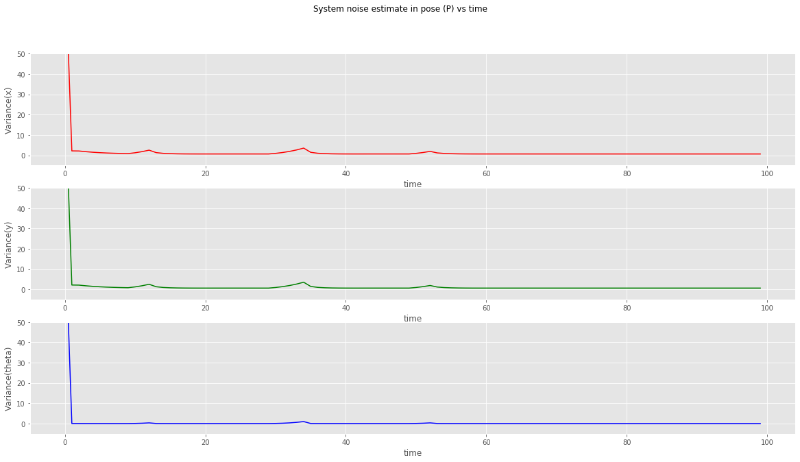
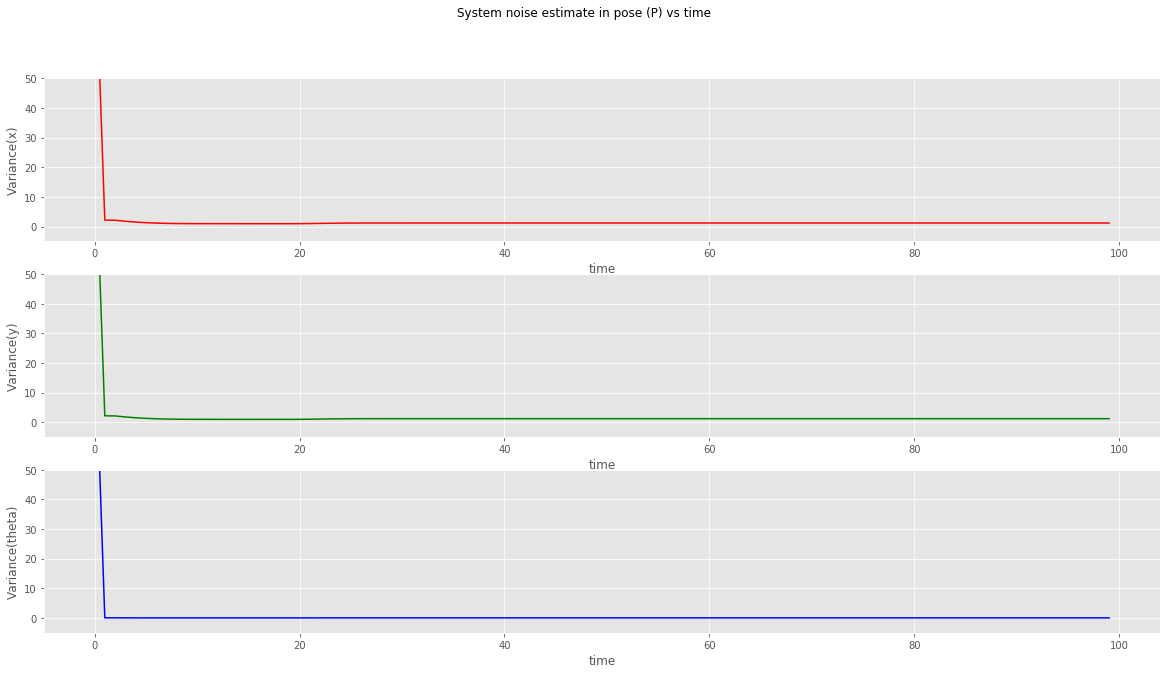
kalman filter (constant velocity model) plot of variances in x, y and theta

The variances at x, y and theta are plotted in the graph above. We can see that when the position data goes missing, the kalman filter will predict the robot position at the same time say that we have now more noise in the system and hence less accuracy in the estimate.
These variances fall back close to zero once the measurements become available.

Kalman Filter (Sensor fusion)

How sensor fusion works

Here a kalman filter is designed that estimates the system state based on 2 sensor inputs (position sensor eg: gps and an acceleration sensor eg: imu)

The state space model here has 3 more states of the robot (acceleration in x, y and theta) as these states will be updated using the imu. $X_{n} = \begin{bmatrix} x_{n} \\ y_{n} \\ \theta_{n} \\ \dot{x}_{n} \\ \dot{y}_{n} \\ \dot{\theta}_{n} \\ \ddot{x}_{n} \\ \ddot{y}_{n} \\ \ddot{\theta}_{n} \end{bmatrix}$
Dynamics matrix $A$ now has the terms for acceleration from equations of motion, matrix $B$ has terms for jerk (the differential of acceleration, check taylor series expansion) in this model but is not used for prediction since we provide no control input matrix $U$ . $B$ will only be used to compute $Q$ matrix.
$A = \begin{bmatrix} 1 & 0 & 0 & t & 0 & 0 & \frac{t^2}{2} & 0 & 0 \\ 0 & 1 & 0 & 0 & t & 0 & 0 & \frac{t^2}{2} & 0 \\ 0 & 0 & 1 & 0 & 0 & t & 0 & 0 & \frac{t^2}{2} \\ 0 & 0 & 0 & 1 & 0 & 0 & t & 0 & 0 \\ 0 & 0 & 0 & 0 & 1 & 0 & 0 & t & 0 \\ 0 & 0 & 0 & 0 & 0 & 1 & 0 & 0 & t \\ 0 & 0 & 0 & 0 & 0 & 0 & 1 & 0 & 0 \\ 0 & 0 & 0 & 0 & 0 & 0 & 0 & 1 & 0 \\ 0 & 0 & 0 & 0 & 0 & 0 & 0 & 0 & 1 \\ \end{bmatrix} \text{ } B = \begin{bmatrix} \frac{t^3}{6} & 0 & 0 \\ 0 & \frac{t^3}{6} & 0 \\ 0 & 0 & \frac{t^3}{6} \\ \frac{t^2}{2} & 0 & 0 \\ 0 & \frac{t^2}{2} & 0 \\ 0 & 0 & \frac{t^2}{2} \\ t & 0 & 0 \\ 0 & t & 0 \\ 0 & 0 & t \end{bmatrix}$
Process noise matrix $Q$ will account for noise in the system due to neglecting jerk and other higher order differentials. The three dots on x, y and theta indicate the third order differential (jerk) accounting for noise in x, y and theta. The values of diagonals are selected as small values in range 0 to 1.
$Q_a = \begin{bmatrix} \sigma_{\dddot{x}}^2 & 0 & 0 \\ 0 & \sigma_{\dddot{y}}^2 & 0 \\ 0 & 0 & \sigma_{\dddot{\theta}}^2 \end{bmatrix}$
We have 2 measurement models in this case has as there are 2 sensors

Position sensor model: needs matrix $H_{pos}$ which has dimensions 3x9 since 3 variables are measured (x, y and theta) and the state has 9 variables. $H_{pos} = \begin{bmatrix} 1 & 0 & 0 & 0 & 0 & 0 & 0 & 0 & 0 \\ 0 & 1 & 0 & 0 & 0 & 0 & 0 & 0 & 0 \\ 0 & 0 & 1 & 0 & 0 & 0 & 0 & 0 & 0 \\ \end{bmatrix}$
The noise model for position sensor is given as $R_{pos} = \begin{bmatrix} \sigma_{x}^2 & 0 & 0 \\ 0 & \sigma_{y}^2 & 0 \\ 0 & 0 & \sigma_{{\theta}}^2 \end{bmatrix}$
IMU sensor model: needs matrix $H_{imu}$ which has dimensions 3x9 since 3 variables are measured, acceleration in x, y and theta and the state has 9 variables.
$H_{imu} = \begin{bmatrix} 0 & 0 & 0 & 0 & 0 & 0 & 1 & 0 & 0 \\ 0 & 0 & 0 & 0 & 0 & 0 & 0 & 1 & 0 \\ 0 & 0 & 0 & 0 & 0 & 0 & 0 & 0 & 1 \\ \end{bmatrix}$
The noise model for IMU is given as $R_{imu} = \begin{bmatrix} \sigma_{\ddot{x}}^2 & 0 & 0 \\ 0 & \sigma_{\ddot{y}}^2 & 0 \\ 0 & 0 & \sigma_{\ddot{\theta}}^2 \end{bmatrix}$

The measurement matrices above $H_{pos}$ , $R_{pos}$ are used to update the kalman filter when position inputs are available to the kalman filter, Matrices $H_{imu}$ , $R_{imu}$ are used when imu data is available. Given these updates the kalman filter can work asynchronously to update the state when a sensor measurement is available.

kalman filter (sensor fusion model) tracking robot position

*animation legend to understand the plots*

The animation above was run on 100 timestamps with position data missing at timestamps 10, 11, 12, 30, 31, 32, 33, 34, 50, 51 and 52, while acceleration data missing at 20, 21, 22, 30, 31, 33 and 34. The initial state was set to x=0, y=0 and theta=0, also the velocities and accelerations of respective variables were set to 0.
The predictions now don't overshoot at the corners as we modelled our system accounting the acceleration. At the corners the system can now react to the deceleration being measured from the imu sensor.
At the discontinuities for position we can see that the robot deviates less from the actual path as we still have an acceleration input coming from the imu sensor.
When acceleration data is missing it can be seen that the robot is still able to keep track of its position as we have gps data coming in. Although the acceleration slightly deviates from the ideal value.
Thus from the above animation we can conclude that having multiple sensors on the system not only improves the overall position estimate but also helps when one of the sensor is not receiving data (eg: say when a car enters the tunnel when we lose gps but the onboard imu and wheel encoders can still help us track its position till we are out of the tunnel).

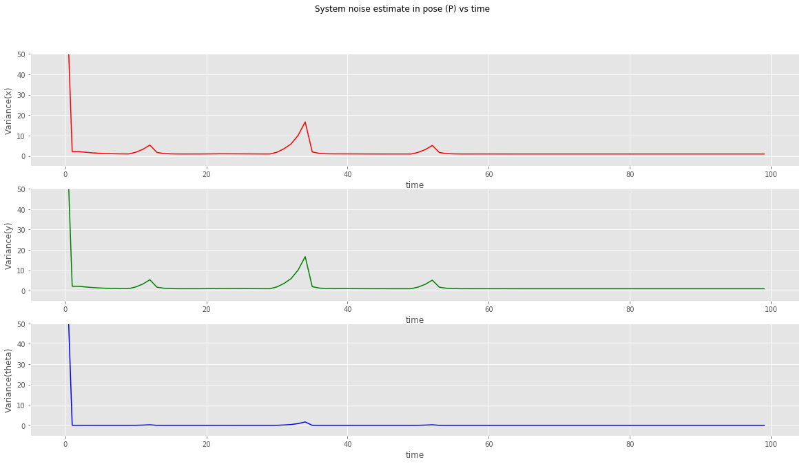
kalman filter (sensor fusion model) plot of variances in x, y and theta

The variances at x, y and theta are plotted in the graph above. When the position data goes missing, the variance increases and falls right back when new position data is available.
When both sensors are switched off individually at different times we can see that the estimate doesn't gather a lot of noise, except when both sensors are both switched off at timestamps 30, 31, 33 and 34 we see that the noise (covariance) increases.

Experiments

In this section we do some experiments with the sensor fusion version of the kalman filter discussed above.

We switch off the imu sensor (acceleration) after 20 timestamps (in real life this could be a failing sensor). The position sensor does keep sending synchronous inputs to the system. The initial state was set to x=0, y=0 and theta=0, also the velocities and accelerations of respective variables were set to 0.

kalman filter (sensor fusion model) tracking robot position with position input only (imu switched off at 20 iterations)
- From the animation we can see that the kalman filter is able to function even though the acceleration input is not available to the system and does a very good job in estimating the acceleration of the robot.
- The acceleration estimate is slightly delayed compared to the true value.
kalman filter (sensor fusion model) plot of variances in x, y and theta
- From the noise estimates of the system it can be seen that the values are slightly higher than actual sensor fusion model.
- At the corners we can see that the noise levels increase which corresponds to the delayed acceleration estimates.

We switch off the position sensor (gps) after 20 timestamps (in real life this could be a failing sensor or a car going into a tunnel losing gps signal). The imu sensor does keep sending synchronous inputs to the system. The initial state was set to x=0, y=0 and theta=0, also the velocities and accelerations of respective variables were set to 0.

kalman filter (sensor fusion model) dead reckoning (position sensor switched off at 20 iterations)
- From the animation we can see that the kalman filter is not able to track the robot right after the position sensor stops sending in data. The estimates do resemble a sine curve as we have acceleration still coming in from the imu.
- The initial offset just before the position sensor switched off will be almost constant in the system since now we never measure position but keep estimating from the last value as is seen from the graph.
- This is called dead reckoning where we try to calculate the robots current position using the previously computed position.
what dead reckoning looks like

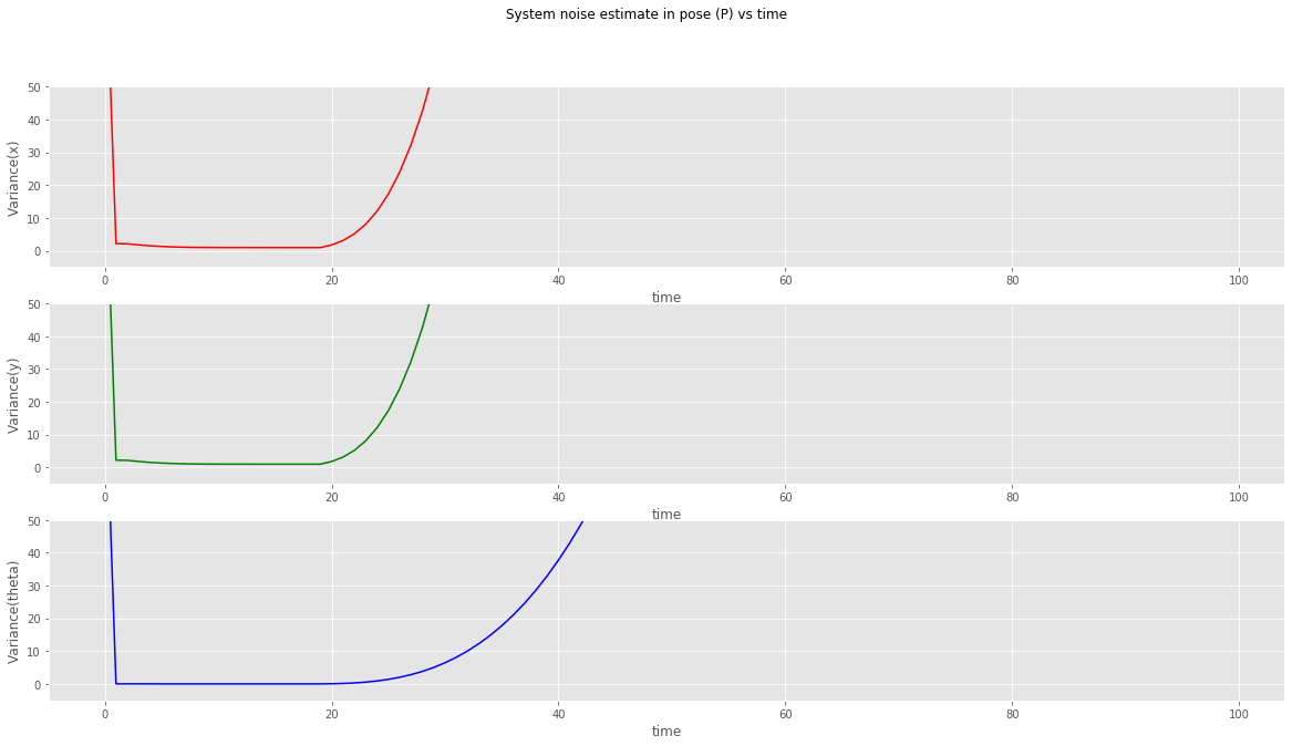
kalman filter (sensor fusion model) plot of variances in x, y and theta
- To compute the position, the acceleration value is integrated twice and hence the noise values add up in the system as can be seen from the variance.
- The errors also rise exponentially immediately after the position sensor is switched off. Which is a good sign as our robot knows how inaccurate its position estimates are.

Design notes

Some key points to keep in mind while designing kalman filters

The Q matrix values should be selected as a value between 0 and 1. the values can be tuned looking at system outputs. The general intuition for Q is, higher the values the less system will trust its prediction as compared to measurements. Q diagonals cannot be set to 0 as this will imply a perfect system giving kalman gain 0 and hence the system will no longer update itself based on measurements rather trust its predictions fully.
The R matrix can be experimentally determined by taking a standard deviation of the error between sensor measurements and true values. This requires a true measurement to be available of the measured quantity, apart from what is measured by the sensor.
Multiple sensors can be fused using the kalman filter given the H and R matrices for those sensors. An update step can be performed when any of the sensor measurements are available.

Source Code

The source code for the tutorial can be found at: https://github.com/MRo47/KalmanFilter

References

Youtube lecture series by Michel van Biezen.
Website with a nice explanation of the single dimensional kalman filter.
LinkedIn tutorial by Mohammad Al-Ahdab.
Video from mathworks on understanding kalman filters

All work

Kalman Filter

A beautiful picture of a lion laughing (maybe) which makes absolutely no sense at all here, just as much sense kalman filter did to me before I decided to write this guide

Introduction

Objectives

Gaussian distribution and product of 2 gaussian PDFs

State estimation using gaussian distribution

Algorithm

Block diagram of kalman filter

Dynamic model

Process noise

Measurement model

Measurement noise

Thank Carl Friedrich Gauss for the normal distribution

Prediction step

Kalman Gain (K)

Correction step

Designing Kalman Filters

Kalman Filter (Constant velocity model)

Legend for animations

kalman filter (constant velocity model) tracking robot position

kalman filter (constant velocity model) plot of variances in x, y and theta

Kalman Filter (Sensor fusion)

How sensor fusion works

kalman filter (sensor fusion model) tracking robot position

kalman filter (sensor fusion model) plot of variances in x, y and theta

Experiments

kalman filter (sensor fusion model) tracking robot position with position input only (imu switched off at 20 iterations)

kalman filter (sensor fusion model) plot of variances in x, y and theta

kalman filter (sensor fusion model) dead reckoning (position sensor switched off at 20 iterations)

what dead reckoning looks like

kalman filter (sensor fusion model) plot of variances in x, y and theta

Design notes

Source Code

References